
Author: Aniruddh

  • Write Rupee Symbol using Keyboard Keys

    Rupee got symbol last year. The font for rupee symbol  is added in Microsoft update. However the manuals do not mention about what are the keys to  use to get  rupee symbol. After searching a lot on internet and manual experiment i got below solution. That is I am able to use rupee symbol ₹ using the key which contains rupee symbol or the keyboards without rupee symbol can use the key with $ symbol. This works for most of the keyboards. Below steps will demonstrate on how to use Rupee symbol (₹). If you want to insert Rupee symbol in Excel, please refer my post on Type  Rupee Symbol in Excel 2010.

    Steps to write Rupee symbol using keyboard:

    • Download the Microsoft driver update which enable the Windows to detect rupee symbol. You can download Microsoft update which supports rupee symbol from here.
    • Download the appropriate version of the update based on your version of Windows.  Once download completes, install the update.
    • In Control Panel, click Clock, Language, and Region, and then click Change keyboards or other input methods.
    • On the Region and Language screen, click Change keyboard on the Keyboards and Languages tab.
    • On the Text Services and Input Languages screen, click Add.
    • On the Add Input Language screen select English (India), and then select the India keyboard check box.
    • Restart the system.
    • Now your keyboard will be able to write rupee symbol.
    • For writing rupee symbol now on wards use Ctrl+Alt+₹(4 or $ on regular key). The Keyboards without rupee symbol, can use Ctrl+Alt+$

    Write Rupee symbol in Dell Laptops

    The method given above works with most of the laptop keyboards and normal keyboards. Recently, I was working on Dell Vostro laptop and above shortcut didn’t worked. In this situation, as mentioned above, you need to change the keyboard layout to India and then use right Alt+$(4). This made me to write rupee symbol on Dell Vostro laptop. Please share you have problems using Rupee symbol in any other keyboards.
    Note:

    • This works with most of the keyboards irrespective whether rupee symbol is present on the key or not. The key with $ will be used to write rupee symbol.
    • Once the rupee support update is installed, we can use rupee currency in excel sheets to as currency format.
    • The using above method to type Rupee symbol using Keyboard key worked well with Logitech Keyboard and Dell Laptop keyboard.
    • Same combination of keys will type rupee symbol in MS Word, Excel or any Microsoft Office documents.

    Incoming Search words:
    Type Rupee Symbol in Keyboard
    How to Type Rupee symbol in Keyboard
    Type Indian Rupee Symbol on keyboard
    Type Rupee Symbol in Dell Keyboard
    Type Rupee Symbol in HP Keyboard

  • Equations in Blogger | CodeCogs Equation Editor

    There are many situations where we need to write equation or quotes of some one in blogger. So writing the formulas with super script in blogger needs little coding. The detailed step by step guide to write equation in blogger is given by codecogs.com.
    To use the subscript and superscript in blogger, we need to take the help of Latex script. To install this script follow the instruction given below.
    Steps to Write equation in Blogger
    Step1:  Open Blogger.com and login.
    Step 2: Go to Layout from the drop down list menu underneath the “More Option” Button.
    Step 3: Within the manage Blogs section, select Design.
    Step 4: On the right hand side, click Add a gadget.
    Step 5: Select the ‘HTML/Javascript’.
    Step 6: Before entering the following text, make sure that you are in ‘Edit HTML’ mode(you are in that mode when that ‘Rich Text’ title is showed in upper right corner), enter the following text into the ‘Content’ area:

    Now select ‘Save’ and exit.Before entering the following text, make sure that you are in ‘Edit HTML’ mode(you are in that mode when that ‘Rich Text’ title is showed in upper right corner), enter the following text into the ‘Content’ area:

    Now select ‘Save’ and exit.
    This script is made to work only convert equations within the …
    and
    You might me thinking why equations found anywhere are not converted, this is dangerous because other scripts may place javascript within your page, which might also contain ‘$’. In particular if you use any jQuery scripts on your page then you’re likely to experience problems.
    Note: If you are using the Dynamic view templates of blogger then, you need to add following script on the end of post while composing in HTML mode.
    Equations in Blogger | CodeCogs Equation Editor:

    Note: Writing equation sin wordpress is very easy. You just need to enable Beautiful Math in jetpack. Using that module you can easily type equation in wordpress blogs.

  • Using Ubuntu Classic Desktop in Ubuntu 11.10

    Ubuntu 11.10 automatically  uses Unity as default session and fall back to 2D for the systems which do not have 3D graphic controllers. To use Ubuntu Classic Desktop(GNOME), you need do little tweaking.

    Steps to be followed to use Ubuntu Classic Desktop(GNOME) in Ubuntu 11.10

    • Open the terminal.  To open terminal, keyboard shortcut is Ctrl+Alt+T
    • In terminal, type sudo apt-get install gnome-session-fallback
    • On completion of installation, restart or log off
    • While logging in back choose GNOME Classic
    • Enjoy the Gnome Classic Session.

  • Creating Templates in Excel

    Excel templates are very useful whenever we need to do repeated tasks. Excel VBA does it. But Excel VBA is a little hard to learn and implement.

    Excel templates is nothing but pre defined format. For example if you want to get Agent productivity report in Excel. You have raw reports which has productive hours, non productive hours and other details. Instead of doing every day look up and sum function, create template. That create a new sheet.  In that put all the fiormula or excel functions and required data. So now onwards whenever you need to do the report, just put the raw reports you will get output immediately.

    Advantages of Excel Templates:

    • Saves lot of time
    • Accuracy of the reports increases as manual work is reduced
    • No need to know complicated VB codes.
    • Get time explore new things
    • Do more analysis on data.
    Useful functions and tools to create Excel Templates: Below are minimum Excel formula you should know to create a simple and effective excel templates.
    • Pivot tables: This is one of the tool very useful. You can customize the data the way you want to. Create calculated fields in pivot table to enhance the look and get more data.
    • Vlookup and Hlookup functions: These lookup functions will be very handy while you need to map some fields based on some data criteria. 
    • Conditional sum and count:  Conditional sum function sumif and conditional count function countif are useful when you need to count or sum of the data for a particular data.
    • Multi conditional sum and count: There are many occasions we need to find sum or count based on multiple criteria. SUMIFS, COUNTIFS and sumproduct are the useful functions
    Tips on Creating Excel Templates:
    • Always create a template such a way that, the output of the template matches with desired report format. Do not give a scope for manual work on template on regular basis. This will save time.
    • Use Conditional functions to get ride of error codes such as #n/a.  For this IF function with iserror function will be very useful.
    • While selecting the range, select only the range you have data. Do not select complete sheet. Selecting whole sheet will slow down the template. Using Dynamic ranges will also helpful.
  • Multi Conditional lookup in Excel

    Have you ever came across a situation wherein you wanted to return a value which matches both row and column? VLOOKUP function in Excel returns the value which is matching the row only. In our previous tutorial, we have shown how to perform two column lookup. In this excel tips post, we will guide you on how to perform multi conditional lookup using match and index functions.

    Limitations of Vlookup:

    • VLOOKUP can be used only if the lookup value is in left of the data which we need to extract from the Table or data.
    • VLOOKUP works with one criteria. That is, lookup value is maximum one.

    Multi Conditional lookup in Excel

    To overcome above-mentioned limitations of VLOOKUP, we can use match and index function of excel to get a result like conditional VLOOKUP.

    Using Match and Index function for conditional lookup

    When Match and index functions of excel used together, we can extract the data from a table irrespective of the weather lookup value is left side or right side of the array. So first let us understand Match and Index functions. To perform conditional lookup, we should understand how match and index functions of excel work.

    Excel Index Function

    Excel Index function returns a value or reference from a table or range.

    Syntax of Excel Index Functions:

    =INDEX(array, row_num, [column_num])

    Explanation of Index Function components

    • Array: Is a range or table where we need to extract the data.
    • row_num: In which row the required value is there.
    • [column_num]: In which column the lookup value is present.

    =INDEX(A1:C5,2,3)  returns 3. We are looking for a data which is 2nd row and 3rd column.

    Excel Match Function

    Match function returns relative position of the specified item is a range of cells.

    Match Function Syntax

    MATCH(lookup_value, lookup_array, [match_type])

    • Lookup_value: The value you need to look up.
    • Lookup_Array: The range where you need to search
    • [match_type]: Match_type can be -1, 0, or 1. It tells Excel how to match the lookup_value to values in the lookup_array.
      • 1 — find the largest value less than or equal to lookup_value (the list must be in ascending order)
      • 0 — find the first value exactly equal to lookup_value. Lookup_array (the list can be in any order)
      • -1 — find the smallest value greater than or equal to lookup_value. (the list must be in descending order)

    Note: If match type is omitted, by default excel consider it as 1.

    Example for Excel Match Function

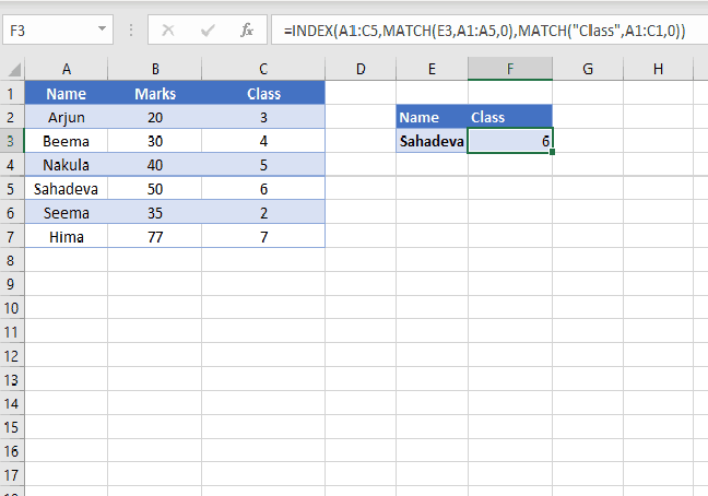
    Consider the same table as above.

    =MATCH(“Sahadeva”,A1:A5,0) returns 5. That is the value “Sahadeva” is in 5th row.

    Using Index and Match together as an alternative to vlookup

    Using index match together will help us in finding 2 criteria lookup and values are present in left of the lookup value.

    Generic Formula

    =INDEX(array, MATCH(lookup_value, lookup_array, [match_type]), MATCH(lookup_value, lookup_array, [match_type]))

    Here what we did is instead of finding row and column numbers we used Match function to find.

    Example:
    =INDEX(A1:C5,MATCH(“Sahadeva”,A1:A5,0),MATCH(“Class”,A1:C1,0)) This returns 6.

    How to MATCH and INDEX work as alternative to VLOOKUP

    We are looking into the table as the range: So, in Index, we used Table as the range. Using Match function, we found rows number of our lookup value “Sahadeva”. For the column number, we once again used Match function to find another criteria column number. That is we are searching for Sahadeva’s Class. So, Class is in 3 row. So, the function returns the value which is in the 5th row and 3rd Column.