

Author: Aniruddh

  • Using Dynamic Named Formula in Excel

    It is a useful concept which saves you a lot of time when you are working with multiple formulas in bigger data range.  The Dynamic named Ranges means the range that isn’t fixed and it can be increased or decreased automatically as per the size of the data. This can be achieved using named ranges feature of Excel without using VBA macros. We will understand this better with a simple example.

    Using Named Formula Ranges in Excel

    Below is the sample data of a sales shop which continuously updates on daily basis.
    Excel Tips and Tricks Examples
    You want to create a name for the data in Column A without referring to empty cells. In simple words, reference to the Dateofpurchase changes every day as you add a new transaction.   In this scenario you can create a dynamic named formula that changes automatically as you enter new data or delete existing data.

    Steps to Create Dynamic Named Formula

    1. Goto Formulas->Defined names-Define Name to display the New Name Dialog box.
    2. Enter DateofPurchase in the Named Field.
    3. Enter the following formula in the  Refers to Field and Click Ok to Close Name Dialog box.

    =OFFSET(Sheet1!$A$2,0,0,COUNTA(Sheet1!$A:$A),1)

    Dynamic Named Formula Creation
    The above step creates a named Formula that uses the excel OFFSET and COUNTA functions to return a range that changes based on the number of non empty cells in column A.To test this let us use a simple COUNTA function

    =COUNTA(Date_Of_Purchase)  

    As you can see, the value changes when you add a new transaction or delete a transaction. This is very useful when you work on large data. Because it uses dynamic memeory allocation, it increases the calculation speed of the formulas. You can see actual difference when you use this with multiple VLOOKUP formula on a large Data range.
    Note:
    The Above shown method works only when you have non empty data range. That is, the range should not contain blanks in between.
  • Handling Error Displays in Excel Formulas

    Sometimes when we use a formula in an Excel worksheet it returns error values such as #N/A, #REF! or #DIV/0!. In some situations we want to know whether the formula returns error values. In some scenarios we do not want to show error values. For example when we create a templates in excel with VLOOKUP, then there will be a error values. To make it look neat, removing error values is an good idea.

    To hide or not to display error values, there primary ISERROR function with IF or direct IFERROR function in Excel 2007 or later will be useful. So let us see simple example so that, you will understand better.

    Different Excel Formulas to Hide Error Values

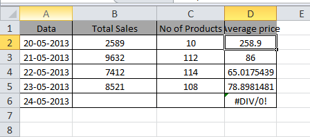
    Below is the sample data and based on this table we will try different ways to hide error messages.

    IF and ISERROR examples
    In the above data, Column D calculates the average price of the products. For this we have used =B2/C2 formula.
    Method 1: Using ISERROR Function with IF condition 
    As you can see from the above table, the formula returns an error if the cells used in the calculation are empty. If you want to hide that error value then use IF function to check an error value using along with ISERROR function. Then the formula becomes
    =if(error(B2/C2),””,B2/C2)
    How it works:
    ISERROR function retunrs true if the argument evaluates to an error.  Then IF function retunrs an empty string otherwise IF function returns the calculated value. You can use this logic with any formula which returns error value such as division, VLOOKUP in Excel etc.
    Using the IFERROR Function
    This formula does the same thing as above. But here it it formula evaluates only once.  This will help you to make your worksheet faster.
    The Formula becomes as below.
    =IFERROR(B2/C2,””)
    Do note that, IFERROR function is first introduced in Excel 2007. So previous versions of excel do not support this function.

  • Steps to Fix Windows 8 Booting Issue after Installing Ubuntu Or Vice Versa

    Today to troubleshoot battery not charging issue due to over heating on my Dell laptop running on Windows 8, I have decided to load the Ubuntu OS onto my system. Ubuntu is known as one of the best free Linux operating system available today. I have downloaded the Ubuntu and installed in a new partition on my hard disk. It got installed properly without any issues. I was able to boot and work on Ubuntu OS. But when I restarted my PC, Windows 8 is not loading! However I was able to boot on Ubuntu. I am new to Ubuntu eco system, so I did research on forums to fixing this problem. My Windows 8 partition is intact and the only problem is, GRUB is not working as expected. After a some 8 to 10 minutes of research on forums, I got a very simple and quick solution to it. So I am sharing the same solution to you which worked for me.

    Steps to Fix Windows 8 Booting Issue after Installing Ubuntu

    Fixing Boot Issues of Windows 8
    Boot-Repair Tool
    To Fix this, there is a simple program called Boot-Repair. It is a small and very useful tool to fix issues such as, you can’t boot Ubuntu after installing Windows or another Linux distribution, or when you can’t boot Windows after installing Ubuntu, or when GRUB is not displayed anymore, some upgrade breaks GRUB, etc.  Below are the steps to fix the boot loader. Ensure you are connected to the Internet before starting below steps.
    1. First you need to install the Boot-Repair Tool. To do this, first open Terminal by pressing Keyboard shortcut Ctrl + ALT + T. In the terminal enter the code given below. (You can copy and paste the code in Terminal. To do so, just copy the codes given below and go to the Terminal, right click on the mouse and select Paste. The Ctrl+V shortcut doesn’t work in Terminal..)

      sudo add-apt-repository ppa:yannubuntu/boot-repair && sudo apt-get update

    It will ask for your admin password. Enter it. It will download all the required repositories. Once it completes , enter the below code in the Terminal.

    sudo apt-get install -y boot-repair && (boot-repair &) 

    2. It will finish installing the Boot-Repair tool.
    3.Launch ‘Boot-repair’ by typing ‘boot-repair‘ in a terminal
    4.Then click the “Recommended repair” button. It will take some time to repair. Once the repair is finished, note the URL (paste.ubuntu.com/XXXXX) that appeared in a paper, then reboot. My problem is resolved at this stage.
    5. If you still face issue then, indicate the URL which you have noted down to people who help you by email or forum which is provided in the last screen of the repair process.

    Steps to Fix Ubuntu Booting Issue after Installing Windows 8

    This one I have not tried. However, I am just quoting the solution provided in the forum. Here  I assume that you have installed Ubuntu first and then installed Windows 8. Now you cannot boot on to Ubuntu. In this case, first boot your computer on a Ubuntu live-CD or live-USB.Then follow the same procedure mentioned above. It updates GRUB and you will be able to access Ubuntu.

  • How to Calculate Service Level In a Inbound Call Center

    The Inbound call center or contact center service level is one of the key factors to track the performance. Though it cannot be defined directly. This is because, the calculation depends on requirements. Some companies consider abandoned calls and some do not consider. In general we can define service level as the number of calls answered within the threshold.  Below is the formula to calculate service level percentage.

    Formula to Calculate Service Level Percentage in Inbound Call Center

    As said above, the formula to calculate changes with company to company. So below is the formula which most of the companies use.

    Service Level %= (Total Calls Answered within threshold/Total Calls Offerred)*100

    The above formula is not considering the abandoned calls. So if you need to consider that, then you should use below formula.

    Service Level %=(Total Calls Offerred-Total Calls Answered after threshold-Total calls abandoned after threshold)/(Total Calls offered-Total calls abandoned within threshold))

    Where
    ‘Total Calls Answered after threshold’ is nothing but the number of calls answered after the target time frame. Depending on the business, each company defines the time. Some may say 20 sec ,10 sec,120 sec etc to answer the call,
    Abandoned after threshold or Within Threshold- This is the calls abandoned within the target time. Some companies do not consider calls which gets abandoned within 10sec or 20 sec. It can be a higher value too.

    Examples on calculating service level % in a Inbound contact center

    In a day, a contact center gets 1000 calls and 40 calls answered after the threshold time of 20 sec. 60 calls got abandoned after threshold of 10 sec and 30 calls within threshold.  What is service level?
    The total calls answered=(1000-30+60)=1030
    Total calls answered within threshold is (910-40)=990
    Service level=(1000-40-60)/(1000-30)=92.78%

  • Excel Formula to Write Date Format In Excel

    In excel we can use a date in different formats according to our wish by clicking on format cells and selecting the required Date format. This works on most of scenarios. But using formula to set the format of date comes handy at times.  So in this Excel tips and tricks guide we will learn to use Excel formula which converts date into desired format.

    Excel Formula to Convert Date in desired Format

    This way of formatting comes very handy when you are using nested function or output of any function which is date. For example you are creating template and sharing with other. They might not be knowing the formatting. So when extend the formula to some other row or column, they will not get the date in desired format. So if you embed the date format in the excel function itself, then it will be more easier. For formating the date in excel using function, text worksheet function is useful. Example is given for such scenario is given in the end of this post.

    Syntax of Text worksheet function

    =text(Date, Date Format)

    Example:
    Let us say, the date is in cell A1, then the formula will be
    =TEXT(A1,”dd-mmm-yyyy”) which returns date in 24-Apr-2013
    =TEXT(A1,”dd-mm-yyyy”) returns date in 24-04-2013 format
    =TEXT(A1,”dd-mmmm-yyyy”)return date as 24-April-2013
    =TEXT(A1,”yyyy”) returns 2013
    =TEXT(A1,”mmmm”) returns April
    Hope you got the concept of using Excel formula to get Date format.  This Excel formula to format date is very useful when you are using date inside or along with another Formula. For example, let us say in cell A1 we have “todays date” and in cell B1 we have 24-April-2013. When we concatenate these two cells, the result shows  todays date41388. To make date to appear in correct formar we need to enter the formula as mentioned below.
    =A1&TEXT(B1,”dd-mmm-yyyy”) which returns todays date24-Apr-2013.
    Please let me know if you need further details on the same.